Stress, Strain and Elastic Constant

Stress :
Mechanical stress can be defined as the force acting on a body per unit area.

In above figure, left figure shows a prismatic bar applied with a load 'P', which develops a total internal resisting force (R) on cross-section, and figure on right shows the free body diagram of left fig. Then the Stess can be define as the magnitude or intensity of internal resisting force developed at a point in a member under given load.

\[ \sigma = \frac{dF}{dA} \] \[ \textrm{ On Integration : } \int{dR} = R = \sigma \int{dA} \] \[ \Rightarrow R = \sigma A \] \[ \boxed{ \sigma_{avg} = \frac{R}{A} = \frac{P}{A} } \] Stress Vs Pressure :

Stress	Pressure
stress magnitude can be different in different direction	Same in every direction
Stress can't be measured	Pressure gauges can be use to measure pressure
Acts normal or along to the applied load	Acts normal to the surface
Stress may be tensile, compressive and shear	Pressure is always compressive
Stress is a Second order tensor	Pressure is a scalar quantity

Zero order tensor :
Zero order tensor are basically Scalar quantity means it has only magnitude.
First order tensor :
First order tensor are basically Vector quantity means it has magnitude and one direction.
Second order tensor :
Second order tensor have both magnitude and 2 direction. Example :- Stress , Strain

\[ \sigma_{[plane][direction]} \]

Engineering Vs True stress

Engineering stress : It is the ratio of applied load at any instant to average original cross-sectional area. Engineering Stress is denoted S or \( \sigma_{e} \).

\[ S = \sigma_{e} = \frac{P}{A_{0}} \]

Where P is applied load and \( A_{0} \) is Avg. Cross-sectional area

True stress : It is the ratio of applied load at any instant to instantaneous cross-sectional area. True Stress is denoted as \( \sigma_{T} \). \[ \sigma_{T} = \frac{P}{A} \] Where P is applied load and \( A \) is instantaneous Cross-sectional area

Units of Stress : Pa ( \( \frac{N}{m^2} \) ) , MPa ( \( 10^6 \frac{N}{m^2} \) = 1MPa ) , \( \frac{kgf}{cm^2} ( 1kgf = 9.81N \Rightarrow 1\frac{kgf}{cm^2} = 0.1MPa ) \)

Relation between True stress and Engineering stress: \[ \sigma_{T} = \sigma_{e}( 1 + e ) \] \( e \) = Engg. Strain
\( \sigma_{e} \) = Engg. Stress
\( \sigma_{T} \) = True Stress

---

Engineering Vs True strain

Engineering strain : It is the ratio of change in dimension to original dimension om application of load. Engineering Strain is denoted e. \[ e = \frac{\Delta L}{L_{0}} \] Where \( \delta L \) is change in dimesion and \( L_{0} \) is original length

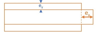
Longitudinal Strain \( (e_{x}) \) : It is the normal strain in the direction of applied load
Lateral Strain \( (e_{y}) \) : It is the normal strain in the direction perpendicular of applied load
    Note :
            (1) Longitudinal Strain and Lateral Strain are always unlike in nature
            (1) Every longitudinal strain is associated with 2 lateral strain

True strain : True strain equals the natural log of the quotient of current length over the original length. True Strain is denoted as \( \epsilon \). \[ \epsilon = \ln{\frac{L}{L_{0}}} = \ln{\frac{A_0}{A}} = \ln{ \frac{1}{1-q} } \] Here,
L₀ and A₀ is intial length and cross-section area respectively
L and A is final length and cross-section area respectively
q = percentage reduction in cross-sectional area

Units of Strain : Dimensionless

Relation between True stran and Engineering strain : \[ \sigma_{T} = \sigma_{e}( 1 + e ) \] \( e \) = Engg. Strain
\( \sigma_{e} \) = Engg. Stress
\( \sigma_{T} \) = True Stress

---

Volume strain :
Volumetric strain is defined as the total change in volume divided by the original volume, i.e., ΔV/V. Let assume a block is strained as \( e_{x} \textrm{ , } e_{y} \textrm{ and, } e_{z}\) in x, y, and z direction respectively. Then volumeric strain will be-


\[ e_{v} = \frac{\Delta V}{V_{0}} = \frac{V_{0}[(1+e_{x})(1+e_{y})(1+e_{z})-1]}{V_{0}} \] \[ e_{v} = (1+e_{x})(1+e_{y})(1+e_{z})-1 \] On neglecting square and Cube term \[ e_{v} = \Delta = e_{x} + e_{y}+ e_{z} \] For Rectengular block : \[ e_{v} = e_{long} + 2 e_{lateral} \]
For Spherical block : \[ e_{v} = 3 \frac{\Delta D}{D} = 3 e_{x} = 3 e_{y} = 3 e_{z} \]

---

Shear strain :

Shear strain is defined as the change in initial right angle between two lines elements which are parallel to x and y axes. The above figure shows the simple shear strain is a combination of pure shear and rotation. Shear strain can be calculated as \( \gamma = \phi^\textrm{shear angle} \) \[ tan\phi^\textrm{shear angle} = \frac{\delta}{L} \] \( \textrm{As }\phi \textrm{ is so small } \Rightarrow \phi = \frac{\delta}{L} \) \[\boxed{ \gamma = \frac{\delta}{L} } \]

---

Elastic Constant

For homogeneous and isotropic material the number of elastic constants are 4. and the number of independent elastic constant are 2 (i.e., \(\mu , E \))

    Elastic Modulus (E) :
\[ E = \frac{\sigma}{e} \]     Modulus of Rigidity (G) :
\[ G = \frac{Shear Stress}{Shear Strain} \]     Bulk Modulus (K) :
\[ K = \frac{\sigma_{hydostatic}}{Vol. Strain} \]     Poission ratio ( \( \mu \) ) : \[ \mu = - \frac{\textrm{Lateral Strain}}{\textrm{Longitudinal Strain}} \]

Material	Independent Elastic Constant
Isotropic	2
Orthotropic	9
Anisotropic	21

    Relationship between elastic constant : \[\boxed{ E = 2G(1 +\mu) }\] \[\boxed{ E = 3K(1-2\mu)} \] \[ \boxed{E = \frac{9KG}{3K + G}} \]    For metals \( \boxed{E > K > G} \)
   Value of Elastic Constants \( \geq 0\)
          E, K, G > 0 and \( \mu \geq 0 \) Ex. \( \mu_{cork} = 0 \)
          From 2nd equation \( 1-2\mu = 0 \Rightarrow \mu \geq \frac{1}{2} \) \[ \boxed{ 0 \leq \mu \leq \frac{1}{2} }\]

Volumetric strain under triaxial state of stress :
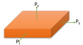
As mentioned earlier , Every longitudinal strain is associated with 2 lateral strain. For above case the longitudinal strain in x-direction \( \frac{\sigma_{x}}{E}\) is associated with 2 lateral strain \( -\frac{\mu \sigma_{x}}{E} \). So for all direction :

\( \frac{Strain \rightarrow}{Load \downarrow} \)	X-Direction	Y-Direction	Z-Direction
Px	\( \frac{\sigma_{x}}{E}\)	\( -\frac{\mu \sigma_{x}}{E} \)	\( -\frac{\mu \sigma_{x}}{E} \)
Py	\( -\frac{\mu \sigma_{y}}{E} \)	\( \frac{\sigma_{y}}{E}\)	\( -\frac{\mu \sigma_{y}}{E} \)
Pz	\( -\frac{\mu \sigma_{z}}{E} \)	\( -\frac{\mu \sigma_{z}}{E} \)	\( \frac{\sigma_{z}}{E}\)

Hence,
Total strain in x-direction \( e_{x} = \frac{1}{E} [\sigma_{x} - \mu(\sigma_{y}+\sigma_{z})] \)
Total strain in x-direction \( e_{y} = \frac{1}{E} [\sigma_{y} - \mu(\sigma_{x}+\sigma_{z})] \)
Total strain in x-direction \( e_{z} = \frac{1}{E} [\sigma_{z} - \mu(\sigma_{x}+\sigma_{y})] \)
As for a rectangular block : \( e_{v} = e_{x} + e_{y} + e_{z} \) \[ \boxed{ e_{v} = \frac{1-2\mu}{E}(\sigma_{x} + \sigma_{y} + \sigma_{z}) } \]